Advanced Statistics and Machine Learning

Quick overview

In this section, we will focus on a practical example to demonstrate the implementations of some advanced statistics, specifically machine learning algorithms, to perform gap filling of eddy covariance data. The concept is to take some gappy data and fill the holes using the meteorological variables associated with the missing values, then compare the methods. It should be noted that we will not go into depth about the statistical methods themselves, but just give an example of the implementation. Indeed, in most cases we will use the default hyper-parameters, which while nice for an overview, is bad practice overall. One should always try to understand a method when implementing it.

required packages

This exercise will require the following packages (all should be available via conda install..., see here for a refresher). If you run into any ModuleNotFoundErrors, don't panic, simply install the missing modules with conda install.:

• numpy

• scipy

• pandas

• scikit-learn

• statsmodels

• xarray

• netcdf4

• dask

Overview of the project

Our sample dataset (provided by me) is a processed eddy covariance file, such as what you would find from the FLUXNET database. If you are unfamiliar with eddy covariance, don't panic, just think of it as a fancy weather station that measures not just meteorological data, but how things come and go from an ecosystem (such as water, energy, and carbon). This file is formatted at a half hourly resolution, so it gives a value for each variable measured every half hour, or 48 points per day (17,520 points per year). One problem with eddy covariance datasets is that they tend to have missing values, or gaps, due to equipment failures or improper measuring conditions. So to fix this, we can predict the missing values, or gap-fill the dataset. This particular dataset has about 40% of the data missing. As we are not the first to deal with gappy eddy covariance datasets, there is a current "standard" method which involves sorting all the values into a look-up table, where values from a similar time-span and meteo conditions are binned, and the gaps are filled with the mean from the bin. We will try to fill the gaps using three statistical methods: random forest, neural networks, and a multi-linear regression.

We will try to organize this project somewhat like you would a real project, which means we will have a number of ".py" files in our project, as well as our data files. So to start, find a nice cozy place in your file system (maybe something like in "Documents" or "MyPyFiles") and create a new folder (maybe called "AdvStat").

In our nice, new, cozy folder, we can first copy the sample dataset, which will be a collection of files that have the file extension ".nc". To keep things tidy, lets put them all in a folder within the folder we created and call it "data". Now we can make three files (maybe don't make them within data), one named "calc.py", one named "regs.py", and one named "plots.py". These files can be created and/or opened into the Spyder IDE to make things a bit easier to work with, or simply in your favorite text editor.

Import and prepare the data

Now, working in the "calc.py" file, we'll start off by importing xarray, with which we can load our data. If we want to open only one file, we could use xr.open_dataset function. Feel free to try opening one file like this:

ds = xr.open_dataset("data/FR-Pue.HH.2003.nc")

Now, we can take a look at how our dataset is organized by simply calling ds in the python interpreter:

ds
↳
<xarray.Dataset>
Dimensions:        (latitude: 1, longitude: 1, time: 262992)
Coordinates:
 * latitude       (latitude) float64 43.74
 * longitude      (longitude) float64 3.596
 * time           (time) datetime64[ns] 2000-01-01T00:15:00 ...
Data variables:
   CO2            (time, latitude, longitude) float32 dask.array<shape=(262992, 1, 1), chunksize=(17568, 1, 1)>
   CO2_QC         (time, latitude, longitude) float32 dask.array<shape=(262992, 1, 1), chunksize=(17568, 1, 1)>
   GPP_DT         (time, latitude, longitude) float32 dask.array<shape=(262992, 1, 1), chunksize=(17568, 1, 1)>
...

Notice the three dimensions and the list of coordinates, followed by the variables and attributes of the dataset. Feel free to play around with the methods you find associated with our ds.

Now, our data is organized in 5 different files, one for each year. Because we want to look at all the data at once, we will be using the xr.open_mfdataset function from xarray, which stands for open multi-file dataset. The syntax looks almost the same, but we replace the file name with a "*", which xr.open_mfdataset will use to mean any file with the ".nc" extension. Give it a try:

import xarray as xr
ds = xr.open_mfdataset('data/*.nc')

Remember that mfdataset means "multi-file dataset", and we are really importing all the ".nc" files in the folder "data". Right away you will want to do two things:

1- the file is three dimensional (time, latitude, and longitude), but as this is only one site, the latitude and longitude dimensions don't change (they have a size of 1), so we can just flatten the array to one dimension using the xr.isel function. xr.isel stands for index selection, so we can give an index of which latitute and longitude we want to select. In this case, because there is only one, this will be 0 in both cases:

ds = ds.isel(latitude=0,longitude=0)

2- you'll want to skip the first year. This is because the first year is only a partial year, so we not only have some gaps in the fluxes, but in all the data, which will mess things up a bit. Thankfully for you, I have been through this dataset and can tell you to skip the first year. In this case, instead of using xr.isel, we will use just xr.sel which will select data by actual values instead of by an index. We can make use of some of xarray's magic and slice the data from 2001 until the end. Since our data goes from 2000 to 2005, and we want to skip the first year, we will take a slice from 2001 to 200......6

ds = ds.sel(time=slice('2001','2006'))

Notice that the dates here are working just like python indexing and does not include the far index, so if we were to use slice('2001','2005') the last year would be left out :(

Now, this netCDF file is fairly well annotated, so if you would like more information on a variable, simply ask:

ds['LE']

You can now see the shape, dimensions, units, and other metadata about this variable.

We will be trying to gap-fill the "LE" variable (Latent Energy, a measure of the water flux), which we can compare to the professionally filled version "LE_f".

As this is a regression problem, we need to get things into an "X" vs "Y" format. For the X variables we will use the following:

XvarList = ['TA','SW_IN','VPD','SW_IN_POT','doy']

Now, if you knew your dataset well, you would know that "doy" (short for day of year) is not yet a variable. Luckily for you, xarray has many nifty features, including the ability to extract time subvariables. We can add "doy" with:

ds['doy'] = ds['time.dayofyear']

You can now check your dataset and all variables should be listed.

With our list of x variables, we can now create a 2 dimensional array in the form number-of-samples by number-of-features. We can do this by first converting the xarray dataset into a numpy array. This is done in two easy steps: first, a built in method of the xarray dataset called .to_array(), which will turn our dataset into a data array which is similar to a numpy array but it still contains the metadata and units. To get rid of all the metadata, we can call another built in method called values, which will really give us just the values, finally in the form of a numpy array. In one line, it looks like this:

X = ds[XvarList].to_array().values

X is now a pure numpy array, but remember that we need it to be shaped like number-of-samples (87648) by number-of-features (5). Check the shape of X. If it is backwards, we will need to transpose the resulting array using the numpy array method .T. If we want to be fancy, we can do everything in one line as:

X = ds[XvarList].to_array().values.T

and like magic we are all ready to go with the Xvars. You can check to make sure we have the right shape again just to be sure.

The Y variable is also easy, as it is simply the array of LE, which if we remember, is stored in our dataset as ds["LE"]. However, we will do a little trick that will seem a bit silly, but will make sense later. Lets first store our Y variable name as a string, then set Y as:

yvarname = "LE"
Y        = ds[yvarname].values

I promise this will come in handy.

Setting up the gapfillers

Now we can move on to our second python file in our cozy folder: "regs.py". This file will hold some of our important functions that help us complete our quest of gapfilling. The only packages to import in this script will be numpy and statsmodels (we'll use statsmodels a bit later).

import numpy as np
import statsmodels.api as sm

Our first function will be quite simple, we just want to be able to find the gaps. Define a function called GapMask which takes ds and yvarname as inputs. As our variable has already been gapfilled once, we need to find the points that weren't original data. In this dataset this information is saved in a companion variable, denoted by the "_QC" at the end of the variable name. So our QC vairable in this case would be "LE_QC". The QC data is an integer between 0 and 3, with 0 being original data and 1, 2, and 3 corresponding to good, medium, and poor quality gapfilling. As we want to deal with only the original data we will want to take all points where LE_QC does not equal 0:

mask = ds[yvarname+'_QC'].values != 0

mask is now a boolean array that says True any time there is a gap and False any time we have original data. Make sure the function is returning the mask!

Our next function will take all the machine learning algorithms that we will use from the SKLearn package and gap fill our dataset, so lets call it "GapFillerSKLearn" and it will take four input variables: X, Y, mask, and model. As this function will be a bit abstract, let add some documentation, which will be a string located immediately after we define the function. I have made an example documentation for our function here:

def GapFillerSKLearn(X,Y,mask,model):
    """
    GapFillerSKLearn(X,Y,mask,model)

    Gap fills Y via X with model

    Uses the provided model to gap fill Y via the X vairiable

    Parameters
    ==========
    X : numpy array
        Predictor variables
    Y : numpy array
        Training set
    mask : numpy boolean array
        array indicating where gaps are with True
    model : regression model from sklearn


    Returns
    =======
    Y_hat
        Gap filled Y as numpy array
    """

Now that the function is documented, we will never forget what this function does.

So we can now move on to the actual function. The reason we can write this function is because the SKLearn module organizes all of it's regressions in the same way, so the method will call "model" whether it is a random forest or a neural net. In all cases we fit the model as:

model.fit(X[~mask],Y[~mask])

where we are fitting only when we don't have gaps. In this case the ~ (tilda) inverts the boolean matrix, making all Trues False and all Falses True, which in our case now gives True to all indices where we have original data. We will be getting mask from GapMask, so remember that it returns True every time LE_Q does not equal 0 (0 is original data). Next we can build our Y_hat variable as an array of NaN values by first creating an array of zeros and multiplying by np.nan. This way if we mess up somewhere in our gapfilling we can see the final values as a NaN. Once we have our NaN array, we can fill Y_hat with all the original data from Y (original data doesn't need to be gap filled).

Y_hat           = np.zeros(Y.shape)*np.nan
Y_hat[~mask]    = Y[~mask]

Now, we can fill the gaps by making a prediction from the model with the Xvars as

Y_hat[mask]     = model.predict(X[mask])

where we are no longer using the tilda (~) because we want the gap indices. Remember to return Y_hat at the end of the function.

Now, the second function will be much like the first except it will build a linear model using statsmodels. Unfortunately we cannot use the same function for the linear model, as statsmodels uses a slightly different syntax (note that SKLearn also has an implementation for linear models, but it's good to be well rounded). The statsmodels function will look strikingly similar to our "GapFillerSKLearn" function, but with some key differences. Let's call it "GapFillerLinear". First, build the documentation just as before, the function will take the same inputs with the exception of model, so only X, Y, and mask. Try to make the appropriate documentation based on the one for "GapFillerSKLearn". Then our function will look like this:

X_ols           = sm.add_constant(X)
Y_hat           = np.zeros(Y.shape)*np.nan
Y_hat[~mask]    = Y[~mask]
model           = sm.OLS(Y[~mask],X_ols[~mask])
results         = model.fit()
Y_hat[mask]     = results.predict(X_ols[mask])

Notice that this new function is very similar to the other one, except we define the model within the function, and we have the function sm.add_constant. Basically, sm.add_constant will add another row to our array that acts as the intercept variable. Another major difference is that the pesky X's and Y's are switched in the fit command, making it too different to adapt for our "GapFillerSKLearn" function. Make sure our function has the correct return!

Our final gap filler will be based on an existing model, which we will estimate the parameters for. The model will be called the "Zhou" model but we won't go into detail about it. Here is the formula:

$LE = a \cdot GPP \cdot VPD^{b}$

where a and b are parameters we will fit to our data. This time, we will need two functions, one for the model and one for the gap filller. The first function we will call "ZhouModel", looks like this:

def ZhouModel(X,a,b):
    x1,x2 = X
    Y     = a * x1 * x2**b
    return(Y)

Note that we are giving the model two X variables, but they are packed into one. This is because the parameter estimation function scipy.optimize.curve_fit needs the model in the format of $f(x, ...)$. Now, our second function is called "GapFillerZhou", it takes GPP, VPD, Y, and mask as arguments and looks like this:

X = np.stack( [GPP,VPD] )
y_hat           = np.zeros(Y.shape)*np.nan
y_hat[~mask]    = Y[~mask]
p0 = (0.25,0.5)
params, cov = curve_fit(ZhouModel, X[:,~mask], Y[~mask], p0=p0)
y_hat[mask] = ZhouModel(X[:,mask],*params)

Some things to note about this function: - we use np.stack to put GPP and VPD together in one X variable - we define p0 which is our initial guess for the parameters that scipy.optimize.curve_fit will use - since the first dimension of X is 2 (because of np.stack), we use [:,mask] to tell the array to use all of the first axes, and mask the second. - notice the *params we pass in the last line, this notation allows us to "unpack" everything contained in params, so it is exactly the same as saying ZhouModel(X[:,mask],params[0],params[1])

This all seems a bit complicated, but focus on the fact that we are fitting the parameters "a" and "b", then using our fitted model to predict our gaps. Make sure our function has the correct return!

Now that our gap fillers are all built, we can move back to our "calc.py" file to do some actual gapfilling.

Actually gapfilling

With X and Y defined and our mask and filling functions built, we can actually do some calculations. For this, we will need to import some more packages, namely:

from sklearn.ensemble import RandomForestRegressor
from sklearn.neural_network import MLPRegressor
import regs

where our random forest (RandomForestRegressor) and neural network (MLPRegressor, or Multi-layer Perceptron) come from the SKLearn package. Of course, regs is our own little package we created. As everything is set up, we can define our mask as:

mask = regs.GapMask(ds,yvarname)

Now we can immediately call our SKLearn gap filler function as:

regs.GapFillerSKLearn(X,Y,mask,RandomForestRegressor())

which will return Y_hat. Now, we will want to save our newly produced data for later so we will add our new gap filling variables to our ds. The syntax to do so looks a little funny at first:

ds[yvarname+'_RF'] = (('time'), regs.GapFillerSKLearn(X,Y,mask,RandomForestRegressor()) )

While the left side of the equal sign looks just like a dictionary, the right side is filled with all sorts of parentheses. The reason for this is we have to tell xarray two things: first the name of the dimensions of the data, which we do with ('time'), and sencond the actual data. Once you have added yvarname+'RF', you can check to see it is contained in our dataset. Now do the same for the MLPRegressor (just remember to change the ds key or it will overwrite LE_RF!). Note that there are many, many options for both RandomForestRegressor and MLPRegressor that should likely be changed, but as this is a quick overview, we will just use the defaults. If you were to add the options, such as increasing to 50 trees in the random forest, it would look like this

RandomForestRegressor(n_estimators=50)

The final step is to run the linear and Zhou models:

ds[yvarname+'_LM'] = (('time'), regs.GapFillerLinear(X,Y,mask) )
ds[yvarname+'_ZU'] = (('time'), regs.GapFillerZhou(ds.GPP_DT.values,ds.VPD.values,Y,mask) )

Now, our script is basically done, and we can actually run it (if in Spyder, just press f5).

Depending on the speed of your computer, it may take a few seconds to run, more than you might want to wait for over and over. Therefor, before we move on to the "plots.py" file, it would be a good idea to save the data so we don't have to run "calc.py" every time. For this, we will use the same netCDF format, because it is really easy to do with xarray. To save our data, we simply export as:

ds.to_netcdf(yvarname+'_GapFills.nc')

You can notice that we saved the file with our yvarname, which you will see can come in handy.

And now the plots!

Now we can finally move on to our "plots.py" file, where we will need regs again, the numpy and xarray packages, as well as pyplot from matplotlib as pl. To start, we will keep things simple and just do a comparison of each gap filling method to the standard LE from the original datafile. After comparing these, we will use a kernel density estimate to look at the distribution of our gap-filled values compared to the real, measured values. Finally, we will look at differences in the mean seasonal cycle of the gap filled points. So in total we will have five figures.

First, we will use the exact same mysterious trick that we have been using where we set the yvarname:

yvarname="LE"

Again, mysterious and will be useful I promise.

Now we will need to load the datafile we just created from "calc.py", just like we did before except it's now in a nice neat file.

ds = xr.open_dataset(yvarname+'_GapFills.nc')

Finally, calculate our gapfilled points mask exactly as you did before in calc.py (hint GapMask).

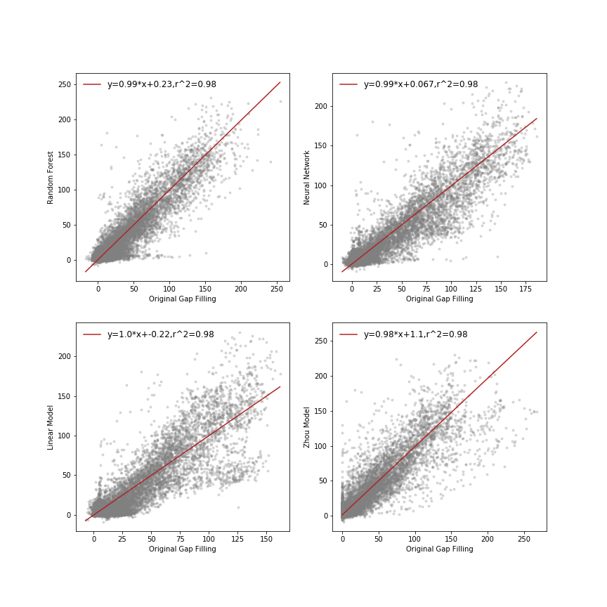
Scatter plots!

As we have three different methods to compare, we can write the plotting steps as a function so we avoid doing all that copy and pasting. Lets call our function "GapComp" and it will take the input variables X, Y, and mask, as well as the optional variable ax:

def GapComp(X,Y,mask,ax=None):

First thing we will do in GapComp is check if ax has been passed, otherwise we will make a new axis:

if ax is None:
    fig,ax = pl.subplots(1)

then we will plot our scatter plot and return our created axis.

ax.scatter(X[mask],Y[mask],marker='.',color='grey',alpha=.25)
return(ax)

You can now try out the plot in the interactive window, plotting LE vs LE_RF:

GapComp(ds.LE_RF.values,ds.LE.values,mask)

Now, we could call it a day, but what fun is a scatter plot without some lines on it. So, we will add the results of a linear regression between our gap filling and the origninal LE using the linregress function from scipy.stats (go ahead and add it to the import list). linregress gives a nice output of a simple linear regression including all the standard stuff. Try running linregress in the interactive window to see what you get:

linregress(ds['LE'],ds['LE_RF'])

Now, we can add a linregress to GapComp:

slope, intercept, r_value, p_value, std_err = linregress(X,Y)

Notice that we got 5 different variables out of one function, how convenient! Remember you can always check the help for a function to see what it will return.

Now that we have fit a model to our models, we can plot our line. To plot, will need an x variable that can we can use to make our line. To do thish we can use the np.linspace command as:

x_line=np.linspace(X[mask].min(),X[mask].max())

Remember you can check the help file of functions if you are not sure what they are doing. And finally, we can plot our line with a nice label showing both our equation and the $r^{2}$ value with

x_line=np.linspace(X[mask].min(),X[mask].max())
ax.plot(x_line,x_line*slope+intercept,color='FireBrick',
        label="y={0:0.2}*x+{1:0.2},r^2={2:0.2}".format(slope, intercept, r_value**2))
ax.legend(frameon=False,loc='upper left', fontsize=12)

And that finishes our function, try it out in the interactive interpreter:

GapComp(ds['LE'].values,ds['LE_RF'].values,mask)

We can now plot all of our models with a neat little for loop:

for var in ["_RF",'_NN','_LM','_ZU']:
    GapComp(ds[yvarname].values,ds[yvarname+var].values,mask)

Now, that gives us a plot, but let's dress it up a bit. First we can make some pretty titles based on our models and store them in a dictionary:

titles = {'_RF':'Random Forest','_NN':'Neural Network','_LM':'Linear Model','_ZU':'Zhou Model'}

Now, with titles defined, we can use it to make some nice lables:

fig,axs = pl.subplots(2,2,figsize=(12,12))
for var,ax in zip(['_RF','_NN','_LM','_ZU'],axs.ravel()):
    GapComp(ds[yvarname+var].values,ds[yvarname].values,mask,ax=ax)
    ax.set_xlabel('Original Gap Filling')
    ax.set_ylabel(titles[var])

Some stats

For the next section, we will convert our xarray dataset to a pandas dataframe. Pandas is a tool built around data tables, so those more familiar with R or excel tables will probably feel more at home with pandas. Luckily, pandas, xarray, numpy, scipy, etc... all work together so we can easily pass objects, functions and methods back and forth. For instance, to make our xarray dataset into a pandas dataframe simply:

df = ds.to_dataframe()

Now you can play with df, and notice how it is the same data but quite different looking. Our time dimension is now a time index, and our different variables now columns. And the difference isn't just in looks, we now have different methods available, try:

df[['LE','LE_RF','LE_NN','LE_LM','LE_ZU']].boxplot()

If you try the same thing with ds, you will get an error because .boxplot is not a method of an xarray dataset. Though they are different objects, the two packages try to keep similar syntax. For instace try the following two lines:

df['LE'].plot()

ds['LE'].plot()

You get almost the same thing, with the major difference being the axis label. Note that both pandas and xarray are using matplotlib in the background, so the plot objects are then identical. In the last few years, the python data science community has really become an ecosystem where packages work together.

For a final exercise, lets test to see if there is a satistical difference between the official gap filling ("LE") and our versions. We should only check the gap filled points, not original points. The test we want to perform is stats.ttest_rel. The results I get are:

LE_RF: mean=22.57 Ttest_relResult(statistic=-3.9933437685851714, pvalue=6.543749693306285e-05)
LE_NN: mean=23.35 Ttest_relResult(statistic=-11.125516920721292, pvalue=1.1990336495569243e-28)
LE_LM: mean=23.44 Ttest_relResult(statistic=-10.048157131446027, pvalue=1.0993508129864383e-23)
LE_ZU: mean=19.86 Ttest_relResult(statistic=17.14875325820577, pvalue=2.444153274115323e-65)

Can you get something close?

Bonus points!

For some bonus points, you can gap fill another variable called "NEE". NEE stands for net ecosystem exchange, and it measures how carbon comes and goes from the ecosystem. Switch out all the times you reference LE (hint, we can finally use the magic trick).